We’re taking the kids to see their favourite band: Muse are playing in Toronto tonight. I’m hoping they play my favourite track:

I find this song fascinating, partly because of the weird mix of progressive rock and dubstep. But more for the lyrics:

All natural and technological processes proceed in such a way that the availability of the remaining energy decreases. In all energy exchanges, if no energy enters or leaves an isolated system, the entropy of that system increases. Energy continuously flows from being concentrated to becoming dispersed, spread out, wasted and useless. New energy cannot be created and high grade energy is destroyed. An economy based on endless growth is unsustainable. The fundamental laws of thermodynamics will place fixed limits on technological innovation and human advancement. In an isolated system, the entropy can only increase. A species set on endless growth is unsustainable.

This summarizes, perhaps a little too succinctly, the core of the critique of our current economy, first articulated clearly in 1972 by the Club of Rome in the Limits to Growth Study. Unfortunately, that study was widely dismissed by economists and policymakers. As Jorgen Randers points out in a 2012 paper, the criticism of the Limits to Growth study was largely based on misunderstandings, and the key lessons are absolutely crucial to understanding the state of the global economy today, and the trends that are likely over the next few decades. In a nutshell, humans exceeded the carrying capacity of the planet sometime in the latter part of the 20th century. We’re now in the overshoot portion, where it’s only possible to feed the world and provide energy for economic growth by consuming irreplaceable resources and using up environmental capital. This cannot be sustained.

In general systems terms, there are three conditions for sustainability (I believe it was Herman Daly who first set them out in this way):

  1. We cannot use renewable resources faster than they can be replenished.
  2. We cannot generate wastes faster than they can be absorbed by the environment.
  3. We cannot use up any non-renewable resource.

We can and do violate all of these conditions all the time. Indeed, modern economic growth is based on systematically violating all three of them, but especially #3, as we rely on cheap fossil fuel energy. But any system that violates these rules cannot be sustained indefinitely, unless it is also able to import resources and export wastes to other (external) systems. The key problem for the 21st century is that we’re now violating all three conditions on a global scale, and there are no longer other systems that we can rely on to provide a cushion – the planet as a whole is an isolated system. There are really only two paths forward: either we figure out how to re-structure the global economy to meet Daly’s three conditions, or we face a global collapse (for an understanding of the latter, see GrahamTurner’s 2012 paper).

A species set on endless growth is unsustainable.

We now have a fourth paper added to our special issue of the journal Geoscientific Model Development, on Community software to support the delivery of CMIP5. All papers are open access:

  • M. Stockhause, H. Höck, F. Toussaint, and M. Lautenschlager, Quality assessment concept of the World Data Center for Climate and its application to CMIP5 data, Geosci. Model Dev., 5, 1023-1032, 2012.
    Describes the distributed quality control concept that was developed for handling the terabytes of data generated from CMIP5, and the challenges in ensuring data integrity (also includes a useful glossary in an appendix).
  • B. N. Lawrence, V. Balaji, P. Bentley, S. Callaghan, C. DeLuca, S. Denvil, G. Devine, M. Elkington, R. W. Ford, E. Guilyardi, M. Lautenschlager, M. Morgan, M.-P. Moine, S. Murphy, C. Pascoe, H. Ramthun, P. Slavin, L. Steenman-Clark, F. Toussaint, A. Treshansky, and S. Valcke, Describing Earth system simulations with the Metafor CIM, Geosci. Model Dev., 5, 1493-1500, 2012.
    Explains the Common Information Model, which was developed to describe climate model experiments in a uniform way, including the model used, the experimental setup and the resulting simulation.
  • S. Valcke, V. Balaji, A. Craig, C. DeLuca, R. Dunlap, R. W. Ford, R. Jacob, J. Larson, R. O’Kuinghttons, G. D. Riley, and M. Vertenstein, Coupling technologies for Earth System Modelling, Geosci. Model Dev., 5, 1589-1596, 2012.
    An overview paper that compares different approaches to model coupling used by different earth system models in the CMIP5 ensemble.
  • S. Valcke, The OASIS3 coupler: a European climate modelling community software, Geosci. Model Dev., 6, 373-388, 2013 (See also the Supplement)
    A detailed description of the OASIS3 coupler, which is used in all the European models contributing to CMIP5. The OASIS User Guide is included as a supplement to this paper.

(Note: technically speaking, the call for papers for this issue is still open – if there are more software aspects of CMIP5 that you want to write about, feel free to submit them!)

Last week, Damon Matthews from Concordia visited, and gave a guest CGCS lecture, “Cumulative Carbon and the Climate Mitigation Challenge”. The key idea he addressed in his talk is the question of “committed warming” – i.e. how much warming are we “owed” because of carbon emissions in the past (irrespective of what we do with emissions in the future). But before I get into the content of Damon’s talk, here’s a little background.

The question of ‘owed’ or ‘committed’ warming arises because we know it takes some time for the planet to warm up in response to an increase in greenhouse gases in the atmosphere. You can calculate a first approximation of how much it will warm up from a simple energy balance model (like the ones I posted about last month). However, to calculate how long it takes to warm up you need to account for the thermal mass of the oceans, which absorb most of the extra energy and hence slow the rate of warming of surface temperatures. For this you need more than a simple energy balance model.

You can do a very simple experiment with a Global Circulation Model, by setting CO2 concentrations at double their pre-industrial levels, and then leave them constant at this level, to see how long the earth takes to reach a new equilibrium temperature. Typically, this takes several decades, although the models differ on exactly how long. Here’s what it looks like if you try this with EdGCM (I ran it with doubled CO2 concentrations starting in 1958):

EVA_time

Of course, the concentrations would never instantaneously double like that, so a more common model experiment is to increase CO2 levels gradually, say by 1% per year (that’s a little faster than how they have risen in the last few decades) until they reach double the pre-industrial concentrations (which takes approx 70 years), and then leave them constant at that level. This particular experiment is a standard way of estimating the Transient Climate Response – the expected warming at the moment we first reach a doubling of CO2 – and is included in the CMIP5 experiments. In these model experiments, it typically takes a few decades more of warming until a new equilibrium point is reached, and the models indicate that the transient response is expected to be a little over half of the eventual equilibrium warming.

This leads to a (very rough) heuristic that as the planet warms, we’re always ‘owed’ almost as much warming again as we’ve already seen at any point, irrespective of future emissions, and it will take a few decades for all that ‘owed’ warming to materialize. But, as Damon argued in his talk, there are two problems with this heuristic. First, it confuses the issue when discussing the need for an immediate reduction in carbon emissions, because it suggests that no matter how fast we reduce them, the ‘owed’ warming means such reductions will make little difference to the expected warming in the next two decades. Second, and more importantly, the heuristic is wrong! How so? Read on!

For an initial analysis, we can view the climate problem just in terms of carbon dioxide, as the most important greenhouse gas. Increasing CO2 emissions leads to increasing CO2 concentrations in the atmosphere, which leads to temperature increases, which lead to climate impacts. And of course, there’s a feedback in the sense that our perceptions of the impacts (whether now or in the future) lead to changed climate policies that constrain CO2 emissions.

So, what happens if we were to stop all CO2 emissions instantly? The naive view is that temperatures would continue to rise, because of the ‘climate commitment’  – the ‘owed’ warming that I described above. However, most models show that the temperature stabilizes almost immediately. To understand why, we need to realize there are different ways of defining ‘climate commitment’:

  • Zero emissions commitment – How much warming do we get if we set CO2 emissions from human activities to be zero?
  • Constant composition commitment – How much warming do we get if we hold atmospheric concentrations constant? (in this case, we can still have some future CO2 emissions, as long as they balance the natural processes that remove CO2 from the atmosphere).

The difference between these two definition is shown here. Note that in the zero emissions case, concentrations drop from an initial peak, and then settle down at a lower level:

Committed-concentrations

CommittedWarming

The model experiments most people are familiar with are the constant composition experiments, in which there is continued warming. But in the zero emissions scenarios, there is almost no further warming. Why is this?

The relationship between carbon emissions and temperature change (the “Carbon Climate Response”) is complicated, because it depends two factors, each of which is complicated by (different types of) inertia in the system:

  • Climate Sensitivity – how much temperature changes in response to difference levels of CO2 in the atmosphere. The temperature response is slowed down by the thermal inertia of the oceans, which means it takes several decades for the earth’s surface temperatures to respond fully to a change in CO2 concentrations.
  • Carbon sensitivity – how much concentrations of CO2 in the atmosphere change in response to different levels of carbon emissions. A significant fraction (roughly half) of our CO2 emissions are absorbed by the oceans, but this also takes time. We can think of this as “carbon cycle inertia” – the delay in uptake of the extra CO2, which also takes several decades. [Note: there is a second kind of carbon system inertia, by which it takes tens of thousands of years for the rest of the CO2 to be removed, via very slow geological processes such as rock weathering.]

Carbon-Response

It turns out that the two forms of inertia roughly balance out. The thermal inertia of the oceans slows the rate of warming, while the carbon cycle inertia accelerates it. Our naive view of the “owed” warming is based on an understanding of only one of these, the thermal inertia of the ocean, because much of the literature talks only about climate sensitivity, and ignores the question of carbon sensitivity.

The fact that these two forms of inertia tend to balance leads to another interesting observation. The models all show an approximately linear response to cumulative emissions. For example, here are the CMIP3 models, used in the IPCC AR4 report (the average of the models, indicated by the arrow, is around 1.6C of warming per 1,000 gigatonnes of carbon):

Temp-Against-Cum-Emissions

The same relationship seems to hold for the CMIP5 models, many of which now include a dynamic carbon cycle:

Temp-against-cum-emissions-CMIP5

This linear relationship isn’t determined by any physical properties of the climate system, and probably won’t hold in much warmer or cooler climates, nor when other feedback processes kick in. So we could say it’s a coincidental property of our current climate. However, it’s rather fortuitous for policy discussions.

Historically, we have emitted around 550 billion tonnes since the beginning of the industrial era, which gives us an expected temperature response of around 0.9°C. If we want to hold temperature rises to be no more than 2°C of warming, total future emissions should not exceed a further 700 billion tonnes of Carbon. In effect, this gives us a total worldwide carbon budget for the future. The hard policy question, of course, is then how to allocate this budget among the nations (or people) of the world in an equitable way.

[A few years ago, I blogged about a similar analysis, which says that cumulative carbon emissions should not exceed 1 trillion tonnes in total, ever. That calculation gives us a smaller future budget of less then 500 billion tonnes. That result came from analysis using the Hadley model, which has one of the higher slopes on the graphs above. Which number we use for a global target then might depend on which model we believe gives the most accurate projections, and perhaps how we also factor in the uncertainties. If the uncertainty range across models is accurate, then picking the average would give us a 50:50 chance of staying within the temperature threshold of 2°C. We might want better odds than this, and hence a smaller budget.]

In the National Academies report in 2011, the cumulative carbon budgets for each temperature threshold were given as follows (note the size of the uncertainty whiskers on each bar):

emissions-targets-NAS2011

[For a more detailed analysis see: Matthews, H. D., Solomon, S., & Pierrehumbert, R. (2012). Cumulative carbon as a policy framework for achieving climate stabilization. Philosophical transactions. Series A, Mathematical, physical, and engineering sciences, 370(1974), 4365–79. doi:10.1098/rsta.2012.0064]

So, this allows us to clear up some popular misconceptions:

The idea that there is some additional warming owed, no matter what emissions pathway we follow is incorrect. Zero future emissions means little to no future warming, so future warming depends entirely on future emissions. And while the idea of zero future emissions isn’t policy-relevant (because zero emissions is impossible, at least in the near future), it does have implications for how we discuss policy choices. In particular, it means the idea that CO2 emissions cuts will not have an effect on temperature change for several decades is also incorrect. Every tonne of CO2 emissions avoided has an immediate effect on reducing the temperature response.

Another source of confusion is the emissions scenarios used in the IPCC report. They don’t diverge significantly for the first few decades, largely because we’re unlikely (and to some extent unable) to make massive emissions reductions in the next 1-2 decades, because society is very slow to respond to the threat of climate change, and even when we do respond, the amount of existing energy infrastructure that has to be rebuilt is huge. In this sense, there is some inevitable future warming, but it comes from future emissions that we cannot or will not avoid. In other words, political, socio-economic and technological inertia are the primary causes of future climate warming, rather than any properties of the physical climate system.

Like most universities, U of T had a hiring freeze for new faculty for the last few years, as we struggled with budget cuts. Now, we’re starting to look at hiring again, to replace faculty we lost over that time, and to meet the needs of rapidly growing student enrolments. Our department (Computer Science) is just beginning the process of deciding what new faculty positions we wish to argue for, for next year. This means we get to engage in a fascinating process of exploring what we expect to be the future of our field, and where there are opportunities to build exciting new research and education programs. To get a new faculty position, our department has to make a compelling case to the Dean, and the Dean has to balance our request with those from 28 other departments and 46 interdisciplinary groups. So the pitch has to be good.

So here’s my draft pitch:

(1) Create a joint faculty position between the Department of Computer Science and the new School of Environment.

Last summer U of T’s Centre for Environment was relaunched as a School of Environment, housed wholly within the Faculty of Arts and Science. As a school, it can now make up to 49% faculty appointments. [The idea is that to do interdisciplinary research, you need a base in a home department/discipline, where your tenure and promotion will be evaluated, but would spend half your time engaged in inter-disciplinary research and teaching at the School. Hence, a joint position for us would be 51% CS and 49% in the School of Environment.]

A strong relationship between Computer Science and the School of Environment makes sense for a number of reasons. Most environmental science research makes extensive use of computational modelling as a core research tool, and the environmental sciences are one of the greatest producers of big data. As an example, the Earth System Grid currently stores more than 3 petabytes of data from climate models, and this is expected to grow to the point where by the end of the decade a single experiment with a climate model would generate an exabyte of data. This creates a number of exciting opportunities for application of CS tools and algorithms, in a domain that will challenge our capabilities. At the same time, this research is increasingly important to society, as we seek to find ways to feed 9 billion people, protect vital ecosystems, and develop strategies to combat climate change.

There are a number of directions we could go with such a collaboration. My suggestion is to pick one of:

  • Climate informatics. A small but growing community is applying machine learning and data mining techniques to climate datasets. Two international workshops have been held in the last two years, and the field has had a number of successes in knowledge discovery that have established its importance to climate science. For a taste of what the field covers, see the agenda of the last CI Workshop.
  • Computational Sustainability. Focuses on the decision-support needed for resource allocation to develop sustainable solutions in large-scale complex adaptive systems. This could be viewed as a field of applied artificial intelligence, but to do it properly requires strong interdisciplinary links with ecologists, economists, statisticians, and policy makers. This growing community has run run an annual conference, CompSust, since 2009, as well as tracks at major AI conferences for the last few years.
  • Green Computing. Focuses on the large environmental footprint of computing technology, and how to reduce it. Energy efficient computing is a central concern, although I believe an even more interesting approach is when we take a systems approach to understand how and why we consume energy (whether in IT equipment directly, or in devices that IT can monitor and optimize). Again, a series of workshops in the last few years has brought together an active research community (see for example, Greens’2013),

(2) Hire more software engineering professors!

Our software engineering group is now half the size it was a decade ago, as several of our colleagues retired. Here’s where we used to be, but that list of topics and faculty is now hopelessly out of date. A decade ago we had five faculty and plans to grow this to eight by now. Instead, because of the hiring freeze and the retirements, we’re down to three. There were a number of reasons we expected to grow the group, not least because for many years, software engineering was our most popular undergraduate specialist program and we had difficulty covering all the teaching, and also because the SE group had proved to be very successful in bringing in research funding, research prizes, and supervising large numbers of grad students.

Where do we go from here? Deans generally ignore arguments that we should just hire more faculty to replace losses, largely because when faculty retire or leave, that’s the only point at which a university can re-think its priorities. Furthermore, some of our arguments for a bigger software engineering group at U of T went away. Our department withdrew the specialist degree in software engineering, and reduced the number of SE undergrad courses, largely because we didn’t have the faculty to teach them, and finding qualified sessional instructors was always a struggle. In effect, our department has gradually walked away from having a strong software engineering group, due to resource constraints.

I believe very firmly that our department *does* need a strong software engineering group, for a number of reasons. First, it’s an important part of an undergrad CS education. The majority of our students go on to work in the software industry, and for this, it is vital that they have a thorough understanding of the engineering principles of software construction. Many of our competitors in N America run majors and/or specialist programs in software engineering, to feed the enormous demand from the software industry for more graduates. One could argue that this should be left to the engineering schools, but these schools tend to lack sufficient expertise in discrete math and computing theory. I believe that software engineering is rooted intellectually in computer science and that a strong software engineering program needs the participation (and probably the leadership) of a strong computer science department. This argument suggests we should be re-building the strength in software engineering that we used to have in our undergrad program, rather than quietly letting it whither.

Secondly, the complexity of modern software systems makes software engineering research ever more relevant to society. Our ability to invent new software technology continues to outpace our ability to understand the principles by which that software can be made safe and reliable. Software companies regularly come to us seeking to partner with us in joint research and to engage with our grad students. Currently, we have to walk away from most of these opportunities. That means research funding we’re missing out on.

I’ve been collecting examples of different types of climate model that students can use in the classroom to explore different aspects of climate science and climate policy. In the long run, I’d like to use these to make the teaching of climate literacy much more hands-on and discovery-based. My goal is to foster more critical thinking, by having students analyze the kinds of questions people ask about climate, figure out how to put together good answers using a combination of existing data, data analysis tools, simple computational models, and more sophisticated simulations. And of course, learn how to critique the answers based on the uncertainties in the lines of evidence they have used.

Anyway, as a start, here’s a collection of runnable and not-so-runnable models, some of which I’ve used in the classroom:

Simple Energy Balance Models (for exploring the basic physics)

General Circulation Models (for studying earth system interactions)

  • EdGCM – an educational version of the NASA GISS general circulation model (well, an older version of it). EdGCM provides a simplified user interface for setting up model runs, but allows for some fairly sophisticated experiments. You typically need to let the model run overnight for a century-long simulation.
  • Portable University Model of the Atmosphere (PUMA) – a planet Simulator designed by folks at the University of Hamburg for use in the classroom to help train students interested in becoming climate scientists.

Integrated Assessment Models (for policy analysis)

  • C-Learn, a simple policy analysis tool from Climate Interactive. Allows you to specify emissions trajectories for three groups of nations, and explore the impact on global temperature. This is a simplified version of the C-ROADS model, which is used to analyze proposals during international climate treaty negotiations.
  • Java Climate Model (JVM) – a detailed desktop assessment model that offers detailed controls over different emissions scenarios and regional responses.

Systems Dynamics Models (to foster systems thinking)

  • Bathtub Dynamics and Climate Change from John Sterman at MIT. This simulation is intended to get students thinking about the relationship between emissions and concentrations, using the bathtub metaphor. It’s based on Sterman’s work on mental models of climate change.
  • The Climate Challenge: Our Choices, also from Sterman’s team at MIT. This one looks fancier, but gives you less control over the simulation – you can just pick one of three emissions paths: increasing, stabilized or reducing. On the other hand, it’s very effective at demonstrating the point about emissions vs. concentrations.
  • Carbon Cycle Model from Shodor, originally developed using Stella by folks at Cornell.
  • And while we’re on systems dynamics, I ought to mention toolkits for building your own systems dynamics models, such as Stella from ISEE Systems (here’s an example of it used to teach the global carbon cycle).

Other Related Models

  • A Kaya Identity Calculator, from David Archer at U Chicago. The Kaya identity is a way of expressing the interaction between the key drivers of carbon emissions: population growth, economic growth, energy efficiency, and the carbon intensity of our energy supply. Archer’s model allows you to play with these numbers.
  • An Orbital Forcing Calculator, also from David Archer. This allows you to calculate what the effect changes in the earth’s orbit and the wobble on its axis have on the solar energy that the earth receives, in any year in the past of future.

Useful readings on the hierarchy of climate models

A high school student in Ottawa, Jin, writes to ask me for help with a theme on the question of whether global warming is caused by human activities. Here’s my answer:

The simple answer is ‘yes’, global warming is caused by human activities. In fact we’ve known this for over 100 years. Scientists in the 19th Century realized that some gases in the atmosphere help to keep the planet warm by stopping the earth losing heat to outer space, just like a blanket keeps you warm by trapping heat near your body. The most important of these gases is Carbon Dioxide (CO2). If there were no CO2 in the atmosphere, the entire earth would be a frozen ball of ice. Luckily, that CO2 keeps the planet at the temperatures that are suitable for human life. But as we dig up coal and oil and natural gas, and burn them for energy, we increase the amount of CO2 in the atmosphere and hence we increase the temperature of the planet. Now, while scientists have known this since the 19th century, it’s only in the last 30 years that scientists were able to calculate precisely how fast the earth would warm up, and which parts of the planet would be affected the most.

Here are three really good explanations, which might help you for your theme:

  1. NASA’s Climate Kids website:
    http://climatekids.nasa.gov/big-questions/
    It’s probably written for kids younger than you, but has really simple explanations, in case anything isn’t clear.
  2. Climate Change in a Nutshell – a set of short videos that I really like:
    http://www.planetnutshell.com/climate
  3. The IPCC’s frequently asked question list. The IPCC is the international panel on climate change, whose job is to summarize what scientists know, so that politicians can make good decisions. Their reports can be a bit technical, but have a lot more detail than most other material:
    http://www.ipcc.ch/publications_and_data/ar4/wg1/en/faqs.html

Also, you might find this interesting. It’s a list of successful predictions by climate scientists. One of the best ways we know that science is right about something is that we are able to use our theories to predict what while happen in the future. When those predictions turn out to be correct, it gives us a lot more confidence that the theories are right: http://www.easterbrook.ca/steve/?p=3031

By the way, if you use google to search for information about global warming or climate change, you’ll find lots of confusing information, and different opinions. You might wonder why that is, if scientists are so sure about the causes of climate change. There’s a simple reason. Climate change is a really big problem, one that’s very hard to deal with. Most of our energy supply comes from fossil fuels, in one way or another. To prevent dangerous levels of warming, we have to stop using them. How we do that is hard for many people to think about. We really don’t want to stop using them, because the cheap energy from fossil fuels powers our cars, heats our homes, gives us cheap flights, powers our factories, and so on.

For many people it’s easier to choose not to believe in global warming than it is to think about how we would give up fossil fuels. Unfortunately, our climate doesn’t care what we believe – it’s changing anyway, and the warming is accelerating. Luckily, humans are very intelligent, and good at inventing things. If we can understand the problem, then we should be able to solve it. But it will require people to think clearly about it, and not to fool themselves by wishing the problem away.

A few weeks back, Randall Munroe (of XKCD fame) attempted to explain the parts of a Saturn V rocket (“Up Goer Five”) using only the most common one thousand words of English. I like the idea, but found many of his phrasings awkward, and some were far harder to understand than if he’d used the usual word.

Now there’s a web-based editor that let’s everyone try their hand at this, and a tumblr of scientists trying to explain their work this way. Some of them are brilliant, but many almost unreadable. It turns out this is much harder than it looks.

Here’s mine. I cheated once, by introducing one new word that’s not on the list, although it’s not really cheating because the whole point of science education is to equip people the right words and concepts to talk about important stuff:

If the world gets hotter or colder, we call that ‘climate’ change. I study how people use computers to understand such change, and to help them decide what we should do about it. The computers they use are very big and fast, but they are hard to work with. My job is to help them check that the computers are working right, and that the answers they get from the computers make sense. I also study what other things people want to know about how the world will change as it gets hotter, and how we can make the answers to their questions easier to understand.

[Update] And here’s a few others that I think are brilliant:

Emily S. Cassidy, Environmental Scientist at University of Minnesota:

In 50 years the world will need to grow two times as much food as we grow today. Meeting these growing needs for food will be hard because we need to make sure meeting these needs doesn’t lead to cutting down more trees or hurting living things. In the past when we wanted more food we cut down a lot of trees, so we could use the land. So how are we going to grow more food without cutting down more trees? One answer to this problem is looking at how we use the food we grow today. People eat food, but food is also used to make animals and run cars. In fact, animals eat over one-third of the food we grow. In some places, animals eat over two-thirds of the food grown! If the world used all of the food we grow for people, instead of animals and cars, we could have 70% more food and that would be enough food for a lot of people!

Anthony Finkelstein, at University College London, explaining requirements analysis:

I am interested in computers and how we can get them to do what we want. Sometimes they do not do what we expect because we got something wrong. I would like to know this before we use the computer to do something important and before we spend too much time and money. Sometimes they do something wrong because we did not ask the people who will be using them what they wanted the computer to do. This is not as easy as it sounds! Often these people do not agree with each other and do not understand what it is possible for the computer to do. When we know what they want the computer to do we must write it down in a way that people building the computer can also understand it.

This week, I start teaching a new grad course on computational models of climate change, aimed at computer science grad students with no prior background in climate science or meteorology. Here’s my brief blurb:

Detailed projections of future climate change are created using sophisticated computational models that simulate the physical dynamics of the atmosphere and oceans and their interaction with chemical and biological processes around the globe. These models have evolved over the last 60 years, along with scientists’ understanding of the climate system. This course provides an introduction to the computational techniques used in constructing global climate models, the engineering challenges in coupling and testing models of disparate earth system processes, and the scaling challenges involved in exploiting peta-scale computing architectures. The course will also provide a historical perspective on climate modelling, from the early ENIAC weather simulations created by von Neumann and Charney, through to today’s Earth System Models, and the role that these models play in the scientific assessments of the UN’s Intergovernmental Panel on Climate Change (IPCC). The course will also address the philosophical issues raised by the role of computational modelling in the discovery of scientific knowledge, the measurement of uncertainty, and a variety of techniques for model validation. Additional topics, based on interest, may include the use of multi-model ensembles for probabilistic forecasting, data assimilation techniques, and the use of models for re-analysis.

I’ve come up with a draft outline for the course, and some possible readings for each topic. Comments are very welcome:

  1. History of climate and weather modelling. Early climate science. Quick tour of range of current models. Overview of what we knew about climate change before computational modeling was possible.
  2. Calculating the weather. Bjerknes’ equations. ENIAC runs. What does a modern dynamical core do? [Includes basic introduction to thermodynamics of atmosphere and ocean]
  3. Chaos and complexity science. Key ideas: forcings, feedbacks, dynamic equilibrium, tipping points, regime shifts, systems thinking. Planetary boundaries. Potential for runaway feedbacks. Resilience & sustainability. (way too many readings this week. Have to think about how to address this – maybe this is two weeks worth of material?)
    • Liepert, B. G. (2010). The physical concept of climate forcing. Wiley Interdisciplinary Reviews: Climate Change, 1(6), 786-802.
    • Manson, S. M. (2001). Simplifying complexity: a review of complexity theory. Geoforum, 32(3), 405-414.
    • Rind, D. (1999). Complexity and Climate. Science, 284(5411), 105-107.
    • Randall, D. A. (2011). The Evolution of Complexity In General Circulation Models. In L. Donner, W. Schubert, & R. Somerville (Eds.), The Development of Atmospheric General Circulation Models: Complexity, Synthesis, and Computation. Cambridge University Press.
    • Meadows, D. H. (2008). Chapter One: The Basics. Thinking In Systems: A Primer (pp. 11-34). Chelsea Green Publishing.
    • Randers, J. (2012). The Real Message of Limits to Growth: A Plea for Forward-Looking Global Policy, 2, 102-105.
    • Rockström, J., Steffen, W., Noone, K., Persson, Å., Chapin, F. S., Lambin, E., Lenton, T. M., et al. (2009). Planetary boundaries: exploring the safe operating space for humanity. Ecology and Society, 14(2), 32.
    • Lenton, T. M., Held, H., Kriegler, E., Hall, J. W., Lucht, W., Rahmstorf, S., & Schellnhuber, H. J. (2008). Tipping elements in the Earth’s climate system. Proceedings of the National Academy of Sciences of the United States of America, 105(6), 1786-93.
  4. Typology of climate Models. Basic energy balance models. Adding a layered atmosphere. 3-D models. Coupling in other earth systems. Exploring dynamics of the socio-economic system. Other types of model: EMICS; IAMS.
  5. Earth System Modeling. Using models to study interactions in the earth system. Overview of key systems (carbon cycle, hydrology, ice dynamics, biogeochemistry).
  6. Overcoming computational limits. Choice of grid resolution; grid geometry, online versus offline; regional models; ensembles of simpler models; perturbed ensembles. The challenge of very long simulations (e.g. for studying paleoclimate).
  7. Epistemic status of climate models. E.g. what does a future forecast actually mean? How are model runs interpreted? Relationship between model and theory. Reproducibility and open science.
    • Shackley, S. (2001). Epistemic Lifestyles in Climate Change Modeling. In P. N. Edwards (Ed.), Changing the Atmosphere: Expert Knowledge and Environmental Government (pp. 107-133). MIT Press.
    • Sterman, J. D., Jr, E. R., & Oreskes, N. (1994). The Meaning of Models. Science, 264(5157), 329-331.
    • Randall, D. A., & Wielicki, B. A. (1997). Measurement, Models, and Hypotheses in the Atmospheric Sciences. Bulletin of the American Meteorological Society, 78(3), 399-406.
    • Smith, L. a. (2002). What might we learn from climate forecasts? Proceedings of the National Academy of Sciences of the United States of America, 99 Suppl 1, 2487-92.
  8. Assessing model skill – comparing models against observations, forecast validation, hindcasting. Validation of the entire modelling system. Problems of uncertainty in the data. Re-analysis, data assimilation. Model intercomparison projects.
  9. Uncertainty. Three different types: initial state uncertainty, scenario uncertainty and structural uncertainty. How well are we doing? Assessing structural uncertainty in the models. How different are the models anyway?
  10. Current Research Challenges. Eg: Non-standard grids – e.g. non-rectangular, adaptive, etc; Probabilistic modelling – both fine grain (e.g. ECMWF work) and use of ensembles; Petascale datasets; Reusable couplers and software frameworks. (need some more readings on different research challenges for this topic)
  11. The future. Projecting future climates. Role of modelling in the IPCC assessments. What policymakers want versus what they get. Demands for actionable science and regional, decadal forecasting. The idea of climate services.
  12. Knowledge and wisdom. What the models tell us. Climate ethics. The politics of doubt. The understanding gap. Disconnect between our understanding of climate and our policy choices.

Last week I was at the 2012 AGU Fall Meeting. I plan to blog about many of the talks, but let me start with the Tyndall lecture given by Ray Pierrehumbert, on “Successful Predictions”. You can see the whole talk on youtube, so here I’ll try and give a shorter summary.

Ray’s talk spanned 120 years of research on climate change. The key message is that science is a long, slow process of discovery, in which theories (and their predictions) tend to emerge long before they can be tested. We often learn just as much from the predictions that turned out to be wrong as we do from those that were right. But successful predictions eventually form the body of knowledge that we can be sure about, not just because they were successful, but because they build up into a coherent explanation of multiple lines of evidence.

Here are the sucessful predictions:

1896: Svante Arrhenius correctly predicts that increases in fossil fuel emissions would cause the earth to warm. At that time, much of the theory of how atmospheric heat transfer works was missing, but nevertheless, he got a lot of the process right. He was right that surface temperature is determined by the balance between incoming solar energy and outgoing infrared radiation, and that the balance that matters is the radiation budget at the top of the atmosphere. He knew that the absorption of infrared radiation was due to CO2 and water vapour, and he also knew that CO2 is a forcing while water vapour is a feedback. He understood the logarithmic relationship between CO2 concentrations in the atmosphere and surface temperature. However, he got a few things wrong too. His attempt to quantify the enhanced greenhouse effect was incorrect, because he worked with a 1-layer model of the atmosphere, which cannot capture the competition between water vapour and CO2, and doesn’t account for the role of convection in determining air temperatures. His calculations were incorrect because he had the wrong absorption characteristics of greenhouse gases. And he thought the problem would be centuries away, because he didn’t imagine an exponential growth in use of fossil fuels.

Arrhenius, as we now know, was way ahead of his time. Nobody really considered his work again for nearly 50 years, a period we might think of as the dark ages of climate science. The story perfectly illustrates Paul Hoffman’s tongue-in-cheek depiction of how scientific discoveries work: someone formulates the theory, other scientists then reject it, ignore it for years, eventually rediscover it, and finally accept it. These “dark ages” weren’t really dark, of course – much good work was done in this period. For example:

  • 1900: Frank Very worked out the radiation balance, and hence the temperature, of the moon. His results were confirmed by Pettit and Nicholson in 1930.
  • 1902-14: Arthur Schuster and Karl Schwarzschild used a 2-layer radiative-convective model to explain the structure of the sun.
  • 1907: Robert Emden realized that a similar radiative-convective model could be applied to planets, and Gerard Kuiper and others applied this to astronomical observations of planetary atmospheres.

This work established the standard radiative-convective model of atmospheric heat transfer. This treats the atmosphere as two layers; in the lower layer, convection is the main heat transport, while in the upper layer, it is radiation. A planet’s outgoing radiation comes from this upper layer. However, up until the early 1930’s, there was no discussion in the literature of the role of carbon dioxide, despite occasional discussion of climate cycles. In 1928, George Simpson published a memoir on atmospheric radiation, which assumed water vapour was the only greenhouse gas, even though, as Richardson pointed out in a comment, there was evidence that even dry air absorbed infrared radiation.

1938: Guy Callendar is the first to link observed rises in CO2 concentrations with observed rises in surface temperatures. But Callendar failed to revive interest in Arrhenius’s work, and made a number of mistakes in things that Arrhenius had gotten right. Callendar’s calculations focused on the radiation balance at the surface, whereas Arrhenius had (correctly) focussed on the balance at the top of the atmosphere. Also, he neglected convective processes, which astrophysicists had already resolved using the radiative-convective model. In the end, Callendar’s work was ignored for another two decades.

1956: Gilbert Plass correctly predicts a depletion of outgoing radiation in the 15 micron band, due to CO2 absorption. This depletion was eventually confirmed by satellite measurements. Plass was one of the first to revisit Arrhenius’s work since Callendar, however his calculations of climate sensitivity to CO2 were also wrong, because, like Callendar, he focussed on the surface radiation budget, rather than the top of the atmosphere.

1961-2: Carl Sagan correctly predicts very thick greenhouse gases in the atmosphere of Venus, as the only way to explain the very high observed temperatures. His calculations showed that greenhouse gasses must absorb around 99.5% of the outgoing surface radiation. The composition of Venus’s atmosphere was confirmed by NASA’s Venus probes in 1967-70.

1959: Burt Bolin and Erik Eriksson correctly predict the exponential increase in CO2 concentrations in the atmosphere as a result of rising fossil fuel use. At that time they did not have good data for atmospheric concentrations prior to 1958, hence their hindcast back to 1900 was wrong, but despite this, their projection for changes forward to 2000 were remarkably good.

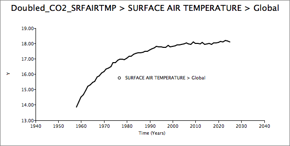
1967: Suki Manabe and Dick Wetherald correctly predict that warming in the lower atmosphere would be accompanied by stratospheric cooling. They had built the first completely correct radiative-convective implementation of the standard model applied to Earth, and used it to calculate a +2C equilibrium warming for doubling CO2, including the water vapour feedback, assuming constant relative humidity. The stratospheric cooling was confirmed in 2011 by Gillett et al.

1975: Suki Manabe and Dick Wetherald correctly predict that the surface warming would be much greater in the polar regions, and that there would be some upper troposphere amplification in the tropics. This was the first coupled general circulation model (GCM), with an idealized geography. This model computed changes in humidity, rather than assuming it, as had been the case in earlier models. It showed polar amplification, and some vertical amplification in the tropics. The polar amplification was measured, and confirmed by Serreze et al in 2009. However, the height gradient in the tropics hasn’t yet been confirmed (nor has it yet been falsified – see Thorne 2008 for an analysis)

1989: Ron Stouffer et. al. correctly predict that the land surface will warm more than the ocean surface, and that the southern ocean warming would be temporarily suppressed due to the slower ocean heat uptake. These predictions are correct, although these models failed to predict the strong warming we’ve seen over the antarctic peninsula.

Of course, scientists often get it wrong:

1900: Knut Angström incorrectly predicts that increasing levels of CO2 would have no effect on climate, because he thought the effect was already saturated. His laboratory experiments weren’t accurate enough to detect the actual absorption properties, and even if they were, the vertical structure of the atmosphere would still allow the greenhouse effect to grow as CO2 is added.

1971: Rasool and Schneider incorrectly predict that atmospheric cooling due to aerosols would outweigh the warming from CO2. However, their model had some important weaknesses, and was shown to be wrong by 1975. Rasool and Schneider fixed their model and moved on. Good scientists acknowledge their mistakes.

1993: Richard Lindzen incorrectly predicts that warming will dry the troposphere, according to his theory that a negative water vapour feedback keeps climate sensitivity to CO2 really low. Lindzen’s work attempted to resolve a long standing conundrum in climate science. In 1981, the CLIMAP project reconstructed temperatures at the last Glacial maximum, and showed very little tropical cooling. This was inconsistent the general circulation models (GCMs), which predicted substantial cooling in the tropics (e.g. see Broccoli & Manabe 1987). So everyone thought the models must be wrong. Lindzen attempted to explain the CLIMAP results via a negative water vapour feedback. But then the CLIMAP results started to unravel, and newer proxies demonstrated that it was the CLIMAP data that was wrong, rather than the models. It eventually turns out the models were getting it right, and it was the CLIMAP data and Lindzen’s theories that were wrong. Unfortunately, bad scientists don’t acknowledge their mistakes; Lindzen keeps inventing ever more arcane theories to avoid admitting he was wrong.

1995: John Christy and Roy Spencer incorrectly calculate that the lower troposphere is cooling, rather than warming. Again, this turned out to be wrong, once errors in satellite data were corrected.

In science, it’s okay to be wrong, because exploring why something is wrong usually advances the science. But sometimes, theories are published that are so bad, they are not even wrong:

2007: Courtillot et. al. predicted a connection between cosmic rays and climate change. But they couldn’t even get the sign of the effect consistent across the paper. You can’t falsify a theory that’s incoherent! Scientists label this kind of thing as “Not even wrong”.

Finally, there are, of course, some things that scientists didn’t predict. The most important of these is probably the multi-decadal fluctuations in the warming signal. If you calculate the radiative effect of all greenhouse gases, and the delay due to ocean heating, you still can’t reproduce the flat period in the temperature trend in that was observed in 1950-1970. While this wasn’t predicted, we ought to be able to explain it after the fact. Currently, there are two competing explanations. The first is that the ocean heat uptake itself has decadal fluctuations, although models don’t show this. However, it’s possible that climate sensitivity is at the low end of the likely range (say 2°C per doubling of CO2), it’s possible we’re seeing a decadal fluctuation around a warming signal. The other explanation is that aerosols took some of the warming away from GHGs. This explanation requires a higher value for climate sensitivity (say around 3°C), but with a significant fraction of the warming counteracted by an aerosol cooling effect. If this explanation is correct, it’s a much more frightening world, because it implies much greater warming as CO2 levels continue to increase. The truth is probably somewhere between these two. (See Armour & Roe, 2011 for a discussion)

To conclude, climate scientist have made many predictions about the effect of increasing greenhouse gases that have proven to be correct. They have earned a right to be listened to, but is anyone actually listening? If we fail to act upon the science, will future archaeologists wade through AGU abstracts and try to figure out what went wrong? There are signs of hope – in his re-election acceptance speech, President Obama revived his pledge to take action, saying “We want our children to live in an America that …isn’t threatened by the destructive power of a warming planet.”

14. November 2012 · 2 comments · Categories: cities

Well here’s an interesting example of how much power a newspaper editor has to change the political discourse. And how powerless actual expertise and evidence is when stacked up against emotive newspaper headlines.

This week, Toronto is removing the bike lanes on Jarvis Street. The removal will a cost around $275,000. These bike lanes were only installed three years ago, after an extensive consultation exercise and environmental assessment that cost $950,000, and a construction cost of $86,000. According to analysis by city staff, the bike lanes are working well, with minimal impact on motor traffic travel times, and a significant reduction of accidents. Why would a city council that claims it’s desperately short of funding, and a mayor who vowed to slash unnecessary spending, suddenly decide to spend this much money removing a successful exercise in urban redesign, against the advice of city staff, against the recommendations of their environmental assessment, and against the wishes of local residents?

The answer is that the bike lanes on Jarvis have become a symbol of an ideological battle.

Up until 2009, Jarvis street had five lanes for motor traffic, with the middle lane working as a ‘tidal’ lane – north in the morning, to accommodate cars entering the city from the Gardiner expressway, and south in the evening when they were leaving. The design never worked very well, was confusing to motorists, and dangerous to cyclists and pedestrians. There was widespread agreement that the fifth lane had to be removed, as part of a much larger initiative to rejuvenate the downtown neighbourhoods along Jarvis Street. The main issue in the public consultation was the question of whether the new design should go for wider sidewalks or bike lanes. After an extensive consultation the city settled on bike lanes, and the vote sailed through council by a large majority.

A few days before the vote, the Toronto Sun, a rightwing and rather trashy tabloid newspaper printed a story under the front page headline “Toronto’s War on the Car“, picking up on a framing for discussions of urban transport that seems to have started with a rather silly rant two years previously in the National Post. The original piece in the National Post was a masterpiece of junk journalism: a story of about a local resident who refuses to take the subway and thinks his commute by car takes too long. Add a clever soundbite headline, avoid any attempt to address the issues seriously, and you’ve manufactured a shock horror story to sell more papers.

The timing of the article in the Toronto Sun was unfortunate – a handful of rightwing councillors picked up the soundbite to and made it a key talking point  in the debate on the Jarvis bike lanes in May 2009. The rhetoric on this supposed ‘war’ quickly replaced any rational discussion of how we accommodate multiple modes of transport, and how we solve urban congestion, and the debate descended into a nasty slanging match about cyclists, with our current mayor (then a councillor), even going so far as to say “bikers are a pain in the ass”.

The National Post upped the rhetoric in its news report the next day:

What started out five years ago as a local plan to beautify Jarvis Street yesterday became the front line in Toronto’s war on the car, with Mayor David Miller leading the charge…

The article never explains what’s wrong with building more bike lanes, but that really doesn’t matter when you have such a great soundbite at your disposal. The idea of a war on the car seems to be a peculiar ‘made in Toronto’ phenomenon, designed to get suburban drivers all fired up and ready to vote for firebrand rightwing politicians, who would then defend their rights to drive whereever and whenever they want. This rhetoric shuts down any sensible discussion about urban planning, transit, and sustainability.

Having seen how well the message played to suburban voters, our current mayor picked up the phrase as a major part of his election campaign, making a pledge to “end Toronto’s war on the car” a key part of his election platform. Nobody was ever clear what that meant, but to the voters in the suburbs, frustrated by their long commutes, it sounded good. Ford evidently believed that it meant cancelling every above-ground transit project currently underway, no matter how much such projects might help to reduce congestion. After his successful election, he declared “We will not build any more rail tracks down the middle of our streets.” Never mind that cities all over the world are turning to surface light rail to reduce congestion and pollution and to improve mobility and liveability. For Ford and his suburban voters, anything that threatens the supremacy of the car as his transport of choice must be stopped.

For a while, the argument transmuted into a debate over subways versus surface-level light rail. Subways, of course, have the benefit that they’re hidden away, so people who dislike mass transit never have to see them, and they don’t take precious street-level space away from cars. Unfortunately, subways are dramatically more expensive to build, and are only cost effective in very dense downtown environments, where they can be justified by a high ridership. Street-level light rail can move many more people at a small fraction of the price, and have the added benefit of integrating transit more tightly with existing streetscapes, making shops and restaurants much more accessible. Luckily for Toronto, sense prevailed, and Mayor Ford’s attempts to cancel Toronto’s plan to build an extensive network of light rail failed earlier this year.

Unfortunately, the price of that embarrassing defeat for Mayor Ford was that something else had to be sacrificed. Politicians need to be able to argue that they delivered on their promises. Having failed to kill Transit City, what else could Ford do but look for an easier win? And so the bike lanes on Jarvis had to go. Their removal will make no noticeable difference to drivers using Jarvis for their commute, and will make the street dramatically less safe for bikes. But Ford gets his symbolic victory. Removing a couple of urban bike lanes is now all that’s left of his promise to end the war on cars.

As Eric de Place points out:

“There’s something almost laughably overheated about the ‘war on cars’ rhetoric. It’s almost as if the purveyors of the phrase have either lost their cool entirely, or else they’re trying desperately to avoid a level-headed discussion of transportation policy.”

Removing downtown bike lanes certainly smacks of a vindictiveness born of desperation.

For a talk earlier this year, I put together a timeline of the history of climate modelling. I just updated it for my course, and now it’s up on Prezi, as a presentation you can watch and play with. Click the play button to follow the story, or just drag and zoom within the viewing pane to explore your own path.

Consider this a first draft though – if there are key milestones I’ve missed out (or misrepresented!) let me know!

”]

We spent some time in my climate change class this week talking about Hurricane Sandy – it’s a fascinating case study of how climate change alters things in complex ways. Some useful links I collected:

In class we looked in detail about the factors that meteorologists look at as a hurricane approaches to forecast likely damage:

  • When will it make landfall? If it coincides with a high tide, that’s far worse than it it comes ashore during low tide.
  • Where exactly will it come ashore? Infrastructure to the north of the storm takes far more damage than infrastructure to the south, because the winds drive the storm surge in an anti-clockwise direction. For Sandy, New York was north of the landfall.
  • What about astronomical conditions? There was a full moon on Monday, which means extra high tides because of the alignment of the moon, earth and sun. That adds inches to the storm surge.

All these factors, combined with the rising sea levels, affected the amount of damage from Sandy. I already wrote about the non-linearity of hurricane damage back in December. After hurricane Sandy, I started thinking about another kind of non-linearity, this time in the impacts of sea level rise. We know that as the ocean warms it expands, and as glaciers around the world melt, the water ends up in the ocean. And sea level sea level rise is usually expressed in measures like: “From 1993 to 2009, the mean rate of SLR amounts to 3.3 ± 0.4 mm/year“. Such measures conjure up images of the sea slowly creeping up the beach, giving us plenty of time to move out of the way. But that’s not how it happens.

We’re used to the idea that an earthquake is a sudden release of the pressure that slowly builds up over a long period of time. Maybe that’s a good metaphor for sea level rise too – it is non-linear in the same way. What really matters about sea level rise isn’t its effects on average low and high tides. What matters is its effect on the height of storm surges. For example, the extra foot added to sea level in New York over the last century was enough to make the difference between the storm surge from Hurricane Sandy staying below the sea walls or washing into the subway tunnels. If you keep adding to sea level rise year after year, what you should expect is, sooner or later, a tipping point where a storm that you could survive previously suddenly become disastrous. Of course, it doesn’t help that Sandy was supersized by warmer oceans, fed by the extra moisture in a warmer atmosphere, and pushed in directions that it wouldn’t normally go by unusual weather conditions over Greenland. But still, it was the exact height of the storm surge that made all the difference, when you look at the bulk of the damage.

”]

The second speaker at our Workshop on City Science was Andrew Wisdom from Arup, talking about Cities as Systems of Systems. Andrew began with the observation that cities are increasingly under pressure, as the urban population continues to grow, and cities struggle to provide adequate infrastructure for their populations to thrive. But a central part of his message is that the way we think about things tends to create the way they are, and this is especially so with how we think about our cities.

As an exercise, he first presented a continuum of worldviews, from Technocentric at one end, to Ecocentric at the other end:

  • In the Techno-centric view, humans are dissociated from the earth. Nature has no inherent value, and we can solve everything with ingenuity and technology. This worldview tends to view the earth as an inert machine to be exploited.
  • In the Eco-centric view, the earth is alive and central to the web of life. Humans are an intrinsic part of nature, but human activity is already exceeding the limits of what the planet can support, to the point that environmental problems are potentially catastrophic. Hence, we need to get rid of materialism, eliminate growth, and work to restore balance.
  • Somewhere in the middle is a Sustain-centric view, which accepts that the earth provides an essential life support system, and that nature has some intrinsic value. This view accepts that limits are being reached, that environmental problems tend to take decades to solve, and that more growth is not automatically good. Humans can replace some but not all natural processes, and we have to focus more on quality of life as a measure of success.

As an exercise, Andrew asked the audience to imagine this continuum spread along one wall of the room, and asked us each to go and stand where we felt we fit on the spectrum. Many of the workshop participants positioned themselves somewhere between the eco-centric and sustain-centric views, with a small cluster at the extreme eco-centric end, and another cluster just to the techno-centric side of sustain-centric. Nobody stood at the extreme techno-centric end of the room!

Then, he asked us to move to where we think the city of Toronto sits, and then where we think Canada sits, and finally where we feel the world sits. For the first two of these, everyone shifted a long way towards the technocentric end of the spectrum (and some discussion ensued to the effect that both our mayor and our prime minister are a long way off the chart altogether – they are both well known for strong anti-environmentalist views). For the whole world, people didn’t move much from the “Canada” perspective. An immediate insight was that we (workshop attendees) are far more towards the ecocentric end of the spectrum than either our current city or federal governments, and perhaps the world in general. So if our governments (and by extension the voters who elect them) are out of step with our own worldviews, what are the implications? Should we, as researchers, be aiming to shift people’s perspectives?

One problem that arises from one’s worldview is how people understand messages about environmental problems. For example, people with a technocentric perspective tend to view discussions of sustainability as being about sacrifice – ‘wearing a hair shirt’, consume less, etc. Which then leads to a waning interest in these topics. For example, analysis of google trends on terms like global warming and climate change show spikes in 2007 around the release of Al Gore’s movie and the IPCC assessment, but declining interest since then.

Jeb Brugmann, the previous speaker, talked about the idea of a Consumptive city versus a Generative city, which is a change in perspective that alters how we view cities, changes what we choose to measure, and hence affects the way our cities evolve.

Changes in the indices we pay attention to can have a dramatic impact. For example, a study in Melbourne created that VAMPIRE index (Vulnerability Assessment for Mortgage, Petroleum and Inflation Risks and Expenses), which shows the relative degree of socio-economic stress in suburbs in Brisbane, Sydney, Melbourne, Adelaide and Perth. The pattern that emerges is that in the Western suburbs of Melbourne, there are few jobs, and many people paying off mortgages, all having to commute and hour and a half to the east of the city for work.

Our view of a city tend to create structures that compartmentalize different systems into silos, and then we attempt to optimize within these silos. For example, zoning laws create chunks of land with particular prescribed purposes, and then we end up trying to optimize within each zone. When zoning laws create the kind of problem indicated by the Melbourne VAMPIRE index, there’s little the city can do about it if they continue to think in terms of zoning. The structure of these silos has become fossilized into the organizational structure of government. Take transport, for example. We tend to look at existing roads, and ask how to widen them to handle growth in traffic; we rarely attempt to solve traffic issues by asking bigger questions about why people choose to drive. Hence, we miss the opportunity to solve traffic problems by changing the relationship between where people live and where they work. Re-designing a city to provide more employment opportunities in neighbourhoods that are suffering socio-economic stress is far more likely to help than improving the transport corridors between those neighbourhoods and other parts of the city.

Healthcare is another example. The outcome metrics typically used for hospital use include average length of stay, 30-day unplanned readmission rate, cost of readmission, etc. Again, these metrics create a narrow view of the system – a silo – that we then try to optimize within. However, if you compare European and American healthcare systems, there are major structural difference. The US system is based on formula funding, in which ‘clients’ are classified in terms of type of illness, standard interventions for that illness, and associated costs. Funding is then allocated to service providers based on this classification scheme. In Europe, service provides are funded directly, and are able to decide at the local level how best to allocate that funding to serve the needs of the population they care for. The European model is a much more flexible system that treats patients real needs, rather than trying to fit each patient into a pre-defined category. In the US, the medical catalogue of disorders becomes an accounting scheme for allocating funds, and the result is that in the US, medical care costs going up faster than any other country. If you plot life expectancy against health spending, the US is falling far behind:

The problem is that the US health system views illness as a problem to be solved. If you think in terms of wellbeing rather than illness, you broaden the set of approaches you can use. For example, there are significant health benefits to pet ownership, providing green space within cities, and so on, but these are not fundable with the US system. There are obvious connections between body mass index and the availability of healthy foods, the walkability of neighbourhoods, and so on, but these don’t fit into a healthcare paradigm that allocates resources according to disease diagnosis.

Andrew then illustrated the power of re-thinking cities as systems-of-systems through several Arup case studies:

  • Dongtan eco-city. This city was designed from the ground up to be food positive, and energy positive (ie. intended to generate more food and more clean energy than it uses). The design makes it more preferable to walk or bike than to drive a car. A key design tool was the use of an integrated model that captures the interactions of different systems within the city. [Dongtan is, incidentally, a classic example of how the media alternately overhypes and then trashtalks major sustainability initiatives, when the real story is so much more interesting].
  • Low2No, Helsinki, a more modest project that aims to work within the existing city to create carbon negative buildings and energy efficient neighbourhoods step by step.
  • Werribee, a suburb of Melbourne, which is mainly an agricultural town, particularly known for its broccoli farming. But with fluctuating prices, farmers have had difficulty selling their broccoli. In an innovative solution that turns this problem into an opportunity, Arup developed a new vision that uses local renewable energy, water and waste re-processing to build a self-sufficient hothouse food production and research facility that provides employment and education along with food and energy.

In conclusion, we have to understand how our views of these systems constrain us to particular pathways, and we have to understand the connections between multiple systems if we want to understand the important issues. In many cases, we don’t do well at recognizing good outcomes, because our worldviews lead us to the wrong measures of success, and then we use these measures to create silos, attempting to optimize within them, rather than seeing the big picture. Understanding the systems, and understanding how these systems shape our thinking is crucial. However, the real challenges then lie in using this understanding to frame effective policy and create effective action.

After Andrew’s talk, we moved into a hands-on workshop activity, using a set of cards developed by Arup called Drivers of Change. The cards are fascinating – there are 189 cards in the deck, each of which summarizes a key issue (e.g. urban migration, homelessness, clean water, climate change, etc), and on the back, distills some key facts and figures. Our exercise was to find connections between the cards – each person had to pick one card that interested him or her, and then team up with two other people to identify how their three cards are related. It was a fascinating and thought-provoking exercise, that really got us thinking about systems-of-systems. I’m now a big fan of the cards and plan to use them in the classroom. (I bought a deck at Indigo for $45, although I note that, bizarrely, Amazon has them selling for over $1000!).

We held a 2-day workshop at U of T last week entitled “Finding Connections – Towards a Holistic View of City Systems“. The workshop brought together a multi-disciplinary group of people from academia, industry, government, and the non-profit sector, all of whom share a common interest in understanding how cities work as systems-of-systems, and how to make our cities more sustainable and more liveable. A key theme throughout the workshop was how to make sure the kinds of research we do in universities does actually end up being useful to decision-makers – i.e. can we strengthen evidence-based policymaking (and avoid, as one of the participants phrased it, “policy-based evidence-making”).

I plan to blog some of the highlights of the workshop, starting with the first keynote speaker.

The workshop kicked off with an inspiring talk by Jeb Brugmann, entitled “The Productive City”. Jeb is an expert in urban sustainability and climate change mitigation, and has a book out called “Welcome to the Urban Revolution: How Cities are Changing the World“. (I should admit the book’s been sitting on the ‘to read’ pile on my desk for a while – now I have to read it!).

Jeb’s central message was that we need to look at cities and sustainability in a radically different way. Instead of thinking of sustainability as about saving energy, living more frugally, and making sacrifices, we should be looking out how we re-invent cities as places that produce resources rather than consume them. And he offered a number of case studies that demonstrate how this is already possible.

Jeb started his talk with the question: How will 9 billion people thrive on Earth? He then took us back to a UN meeting in 1990, the World Congress of Local Governments for a Sustainable Future. This meeting was the first time that city governments around the world came together to grapple with the question of sustainable development. To emphasis how new this was, Jeb recollected lengthy discussions at the meeting on basic questions such as how to translate the term ‘sustainable development’ into French, German, etc.

The meeting had two main outcomes:

  • Initial work on Agenda 21, getting communities engaged in collaborative sustainable decision making. [Note: Agenda 21 was subsequently adopted by 178 countries at the Rio Summit in 1992. More interestingly, if you google for Agenda 21 these days, you’re likely to find a whole bunch of nutball right-wing conspiracy theories about it being an agenda to destroy American freedom.]
  • A network of city governments dedicated to developing action on climate change [This network became ICLEI – Local Governments for Sustainability]. Jeb noted how the ambitions of the cities participating in ICLEI have grown over the years. Initially, many of these cities set targets around 20% reduction in greenhouse gas emissions. Over the years since, these target have grown. For example, Chicago now has a target of 80% reduction. This is significant because these targets have been through city councils, and have been discussed and agreed on by those councils.

An important idea arising out of these agreements is the concept of the ecological footprint – sometimes expressed as how many earths are needed to support us if everyone had the same resource consumption as you. The problem is that you get into definitional twists on how you measure this, and that gets in the way of actually using it as a productive planning tool.

Here’s another way of thinking about the problem. Cities currently have hugely under-optimized development patterns. For example, cities with seven times more outspill growth (suburban sprawl) compared to infill growth. But there are emergent pressures on industry to optimize use of urban space and urban geography. Hence, we should start to examine under-used urban assets. If we can identify space within the city that doesn’t generate value, we can reinvent it. For example, the laneways of Melbourne, which in the 1970’s and 80’s were derelict, have now been regenerated for a rich network of local stores and businesses, and ended up as a major tourist attraction.

We also tend to dramatically underestimate the market viability of energy efficient, sustainable buildings. For example, in Hannover, a successful project built an entire division of eco-homes using Passivhaus standards at similar rental price to the old 1960s apartment buildings.

The standard view of cities, built into the notion of ecological footprint, is that cities are extraction engines – the city acts as a machine that extracts resources from the surrounding environment, processes these resources to generate value, and produces waste products that must be disposed of. Most work on sustainable cities frames the task as an attempt to reduce the impact of this process, by designing eco-efficient cities. For example, the use of secondary production (e.g. recycling) and designed dematerialization (reduction of waste in the entire product lifecycle) to reduce the inflow of resources and the outflow of wastes.

Jeb argues a more audacious goal is needed: We should transform our cities into net productive systems. Instead of focussing on reducing the impact of cities, we should use urban ecology and secondary production so that the city becomes a net positive resource generator. This is far more ambitious than existing projects that aim to create individual districts that are net zero (e.g. that produce as much energy as they consume, through local solar and wind generation). The next goal should be productive cities: cities that produce more resources than they consume; cities that process more waste than they produce.

Jeb then went on to crunch the numbers for a number of different types of resource (energy, food, metals, nitrogen), to demonstrate how a productive city might fill the gap between rising demand and declining supply:

Energy demand. Current European consumption is around 74GJ/capita. Imagine by 2050, we have 9 billion people on the planet, all living like Europeans do now – we’ll need 463EJ to supply them all. Plot this growth in demand over time, and you have a wedge analysis. Using IEA numbers of projected growth in renewable energy supply, to provide the wedges, there’s still a significant shortfall. We’ll need to close the gap via urbanrenewable energy generation, using community designs of the type piloted in Hannover. Cities have to become net producers of energy.

Here’s the analysis (click each chart for full size):

Food. We can do a similar wedge analysis for food. Current food production globally produces around 2,800kcal/captia. But as the population grows, this current level of production produces steadily less food per person. Projected increases in crop yields, crop intensity, and conversion of additional arable land, and reduction of waste would still leave a significant gap if we wish to provide a comfortable 3100kcal/capita. While urban agriculture is unlikely to displace rural farm production, it can play a crucial role in closing the gap between production and need, as the population grows. For example, Havana has a diversified urban agriculture that supplies close to 75% of vegetables from within the urban environment. Vancouver has been very strategic about building its urban agricultural production, with one out of every seven jobs in Vancouver in food production.

Other examples include landfill mining to produce iron and other metals, and urban production of nitrogen fertilizer from municipal biosolids.

In summary, we’ve always underestimated just how much we can transform cities. While we remain stuck in a mindset that cities are extraction engines, we will miss opportunities for more radical re-imagings of the role of global cities. So a key research challenge is to develop a new post-“ecological footprint” analysis. There are serious issues of scaling and performance measurement to solve, and at every scale there are technical, policy, and social challenges. But as cities house ever more of the growing population, we need this kind of bold thinking.

My first year seminar course, PMU199 Climate Change: Software, Science and Society is up and running again this term. The course looks at the role of computational models in both the science and the societal decision-making around climate change. The students taking the course come from many different departments across arts and science, and we get to explore key concepts in a small group setting, while developing our communication skills.

As an initial exercise, this year’s cohort of students have written their first posts for the course blog (assignment: write a blog post on any aspect of climate change that interests you). Feel free to comment on their posts, but please keep it constructive – the students get a chance to revise their posts before we grade them (and if you’re curious, here’s the rubric).

Incidentally, for the course this year, I’ve adopted Andrew Dessler’s new book, Introduction to Modern Climate Change as the course text. The book was just published earlier this year, and I must say, it’s by far the best introductory book on climate science that I’ve seen. My students tell me they really like the book (despite the price), as it explains concepts simply and clearly, and they especially like the fact that it covers policy and society issues as well as the science. I really like the discussion in chapter 1 on who to believe, in which the author explains that readers ought to be skeptical of anyone writing on this topic (including himself), and then lays out some suggestions for how to decide who to believe. Oh, and I love the fact that there’s an entire chapter later in the book devoted to the idea of exponential growth.