Serendipity

This week, I’m featuring some of the best blog posts written by the students on my first year undergraduate course, PMU199 Climate Change: Software, Science and Society. This post is by Harry, and it first appeared on the course blog on January 29.

Projections from global climate models indicate that continued 21^st century increases in emissions of greenhouse gases will cause the temperature of the globe to increase by a few degrees. These global changes in a few degrees could have a huge impact on our planet. Whether a few global degrees cooler could lead to another ice age, a few global degrees warmer enables the world to witness more of nature’s most terrifying phenomenon.

According to Anthony D. Del Genio the surface of the earth heats up from sunlight and other thermal radiation, the amount of energy accumulated must be offset to maintain a stable temperature. Our planet does this by evaporating water that condenses and rises upwards with buoyant warm air. This removes any excess heat from the surface and into higher altitudes. In cases of powerful updrafts, the evaporated water droplets easily rise upwards, supercooling them to a temperature between -10 and -40°C. The collision of water droplets with soft ice crystals forms a dense mixture of ice pellets called graupel. The densities of graupel and ice crystals and the electrical charges they induce are two essential factors in producing what people see as lightning.

Ocean and land differences in updrafts also cause higher lightning frequencies. Over the course of the day, heat is absorbed by the oceans and hardly warms up. Land surfaces, on the other hand, cannot store heat and so they warm significantly from the beginning of the day. The great deal of the air above land surfaces is warmer and more buoyant than that over the oceans, creating strong convective storms as the warm air rises. The powerful updrafts, as a result of the convective storms, are more prone to generate lightning.

According to the general circulation model by Goddard Institute for Space Studies, one of the two experiments conducted indicates that a 4.2°C global warming suggests an increase of 30% in global lightning activity. The second experiment indicated that a 5.9°C global cooling would cause a 24% decrease in global lightning frequencies. The summaries of the experiments signifies a 5-6% change in global lightning frequency for every 1°C of global warming or cooling.

As 21^st century projections of carbon dioxide and other greenhouse gases emission remain true, the earth continues to warm and the ocean evaporates more water. This is largely because the drier land surface is unable to evaporate water at the same extent as the oceans, causing the land to warm more. This should cause stronger convective storms and produce higher lightning occurrence.

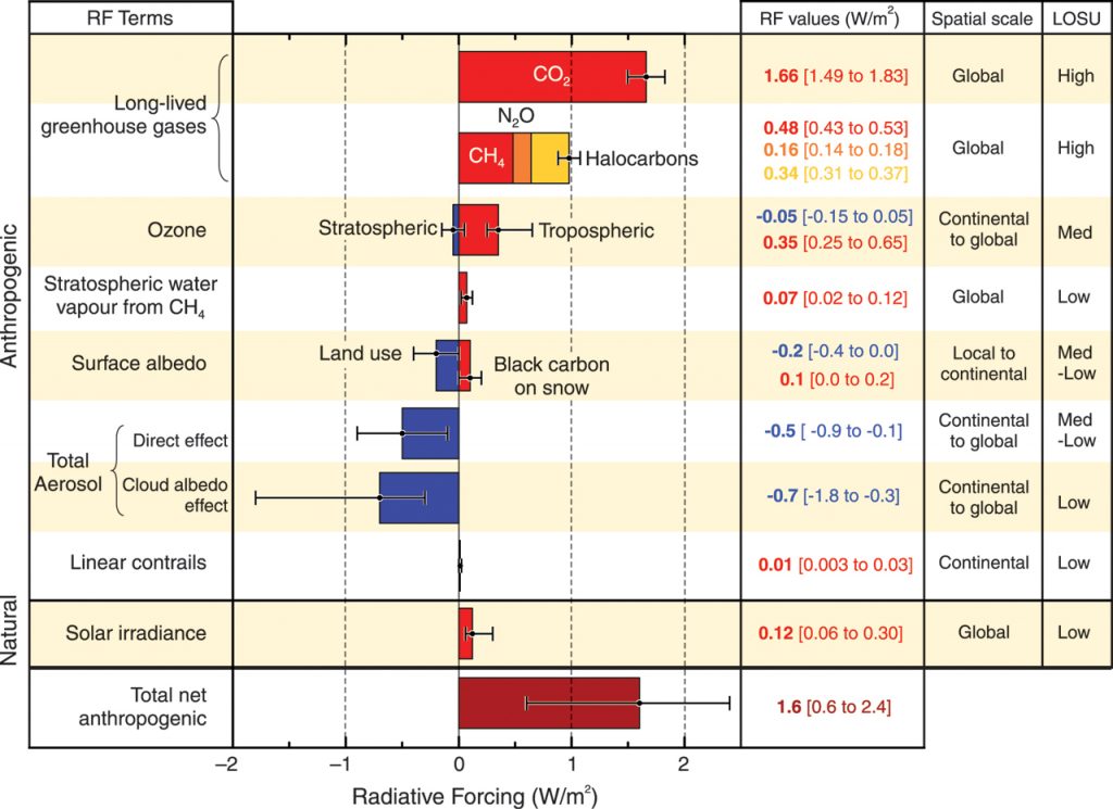
Greater lightning frequencies can contribute to a warmer earth. Lightning provides an abundant source of nitrogen oxides, which is a precursor for ozone production in the troposphere. The presence of ozone in the upper troposphere acts as a greenhouse gas that absorbs some of the infrared energy emitted by earth. Because tropospheric ozone traps some of the escaping heat, the earth warms and the occurence of lightning is even greater. Lightning frequencies creates a positive feedback process on our climate system. The impact of ozone on the climate is much stronger than carbon, especially on a per-molecule basis, since ozone has a radiative forcing effect that is approximately 1,000 times as powerful as carbon dioxide. Luckily, the presence of ozone in the troposphere on a global scale is not as prevalent as carbon and its atmospheric lifetime averages to 22 days.

"Climate simulations, which were generated from four Global General Circulation Models (GCM), were used to project forest fire danger levels with relation to global warming."

Lightning occurs more frequently around the world, however lightning only affects a very local scale. The  local effect of lightning is what has the most impact on people. In the event of a thunderstorm, an increase in lightning frequencies places areas with high concentration of trees at high-risk of forest fire. Such areas in Canada are West-Central and North-western woodland areas where they pose as major targets for ignition by lightning. In fact, lightning accounted for 85% of that total area burned from 1959-1999. To preserve habitats for animals and forests for its function as a carbon sink, strenuous pressure on the government must be taken to ensure minimized forest fire in the regions. With 21st century estimates of increased temperature, the figure of 85% of area burned could dramatically increase, burning larger lands of forests. This is attributed to the rise of temperatures simultaneously as surfaces dry, producing more “fuel” for the fires.

Although lightning has negative effects on our climate system and the people, lightning also has positive effects on earth and for life. The ozone layer, located in the upper atmosphere, prevents ultraviolet light from reaching earth’s surface. Also, lightning causes a natural process known as nitrogen fixation. This process has a fundamental role for life because fixed nitrogen is required to construct basic building blocks of life (e.g. nucleotides for DNA and amino acids for proteins).

Lightning is an amazing and natural occurrence in our skies. Whether it’s a sight to behold or feared, we’ll see more of it as our earth becomes warmer.

A number of sessions at the AGU meeting this week discussed projects to improve climate literacy among different audiences:

• The Climate Literacy and Energy Awareness Network (CLEANET), are developing concept maps for use in middle school and high school, along with a large set of pointers to educational resources on climate and energy for use in the classroom.
• The Climate Literacy Zoo Education Network (CliZEN). Michael Mann (of Hockey Stick Fame) talked about this project, which was a rather nice uplifting change from hearing about his experiences with political attacks on his work. This is a pilot effort, currently involving ten zoos, mainly in the north east US. So far, they have completed a visitor survey across a network of zoos, plus some aquaria, exploring the views of visitors on climate change, using the categories of the Six Americas report. The data they have collected show that zoo visitors tend to be more skewed towards the “alarmed” category compared to the general US population. [Incidentally, I’m impressed with their sample size: 3,558 responses. The original Six Americas study only had 981, and most surveys in my field have much smaller sample sizes]. The next steps in the project are to build on this audience analysis to put together targeted information and education material that links what we know about climate climate with it’s impact on specific animals at the zoos (especially polar animals).
• The Climate Interpreter Project. Bill Spitzer from the New England Aquarium talked about this project. Bill points out that aquaria (and museums, zoos etc) are have an important role to play, because people come for the experience, which must be enjoyable, but they do expect to learn something, and they do trust museums and zoos to provide them accurate information. This project focusses on the role of interpreters and volunteers, who are important because they tend to be more passionate, more knowledgeable, and come into contact with many people. But many interpreters are not yet comfortable in talking about issues around climate change. They need help, and training. Interpretation isn’t just transmission of information. It’s about translating science in a way that’s meaningful and resonates with an audience. It requires a systems perspective. The strategy adopted by this project is to begin with audience research, to understand people’s interests and passions; connect this with the cognitive and social sciences on how people learn, and how they make sense of what they’re hearing; and finally to make use of strategic framing, which gets away from the ‘crisis’ frame that dominates most news reporting (on crime, disasters, fires), but which tends to leave people feeling overwhelmed, which leads them to treat it as someone else’s problem. Thinking explicitly about framing allows you to connect information about climate change with people’s values, with what they’re passionate about, and even with their sense of self-identity. The website climateinterpreter.org describes what they’ve learnt so far
  (As an aside, Bill points out that it can’t just be about training the interpreters – you need institutional support and leadership, if they are to focus on a controversial issue. Which got me thinking about why science museums tend to avoid talking much about climate change – it’s easy for the boards of directors to avoid the issue, because of worries about whether it’s politically sensitive, and hence might affect fundraising.)
• The WorldViews Network. Rachel Connolly from Nova/WGBH presented this collaboration between museums, scientists and TV networks. Partners include planetariums and groups interested in data visualization, GIS data, mapping, many from an astronomy background. Their 3-pronged approach, called TPACK, identifies three types of knowledge: technological, pedagogical, and content knowledge.  The aim is to take people from seeing, to knowing, to doing. For example, they might start with a dome presentation, but bring into it live and interactive web resources, and then move on to community dialogues. Storylines use visualizations that move seamlessly across scale: cosmic, global, bioregional. They draw a lot on the ideas from Rockstrom’s planetary boundaries, within which they’r focussing on three: climate, biodiversity loss and ocean acidification. A recent example from Denver, in May, focussed on water. On the cosmic scale, they look at where water comes from as planets are formed. They eventually bring this down to the bioregional scale, looking at the rivershed for Denver, and the pressures on the Colorado River. Good visual design is a crucial part of the project (Rachel showed a neat example of a visualization of the size of water on the planet: comparing all water, with fresh water and frozen water. Another fascinating example was a satellite picture of the border of Egypt and Israel, where the different water management strategies either side of the border produce a starkly visible difference either side of the border. (Rachel also recommended Sciencecafes.org and the Buckminster Fuller Challenge).
• ClimateCommunication.org. There was a lot of talk through the week about this project, led by Susan Hassol and Richard Somerville, especially their recent paper in Physics Today, which explores the use of jargon, and how it can mislead the general public. The paper went viral on the internet shortly after it was published, and and they used an open google doc to collect many more examples. Scientists are often completely unaware the non-specialists have different meaning for jargon terms, which can  then become a barrier for communication. My favourite examples from Susan’s list are “aerosol”, which to the public means a spray can (leading to a quip by Glenn Beck who had heard that aerosols cool the planet); ‘enhanced’, which the public understands as ‘made better’ so the ‘enhanced greenhouse effect’ sounds like a good thing, and ‘positive feedback’ which also sounds like a good thing, as it suggests a reward for doing something good.
• Finally, slightly off topic, but I was amused by the Union of Concerned Scientists’ periodic table of political interferences in science.